Accidental Taxonomists: When Protein Models Learn the Wrong Shortcut

A protein interaction model is supposed to answer a biological question: are these two proteins likely to bind? In a multi-species dataset, it can quietly be handed a much easier one: did these two proteins come from the same organism?

That substitution is the accidental taxonomist problem. Nobody designs it in. It emerges from a reasonable-looking decision about how to build negative examples, and protein language models are very well equipped to exploit it.

Where the shortcut comes from

Curated interaction databases are positive-first. They record pairs that have been observed to interact. They almost never record pairs that have been tested and found not to interact, because that is not what most papers report. Negatome, the main curated source of real negatives, contributes about 6,000 non-interacting pairs across all of its splits, against hundreds of thousands of positives elsewhere.

So the standard workaround is to manufacture negatives by pairing proteins that are not known to interact. This is defensible. Most protein pairs really do not interact, so a random pair is very likely a true negative.

The trouble is what else changes when you shuffle.

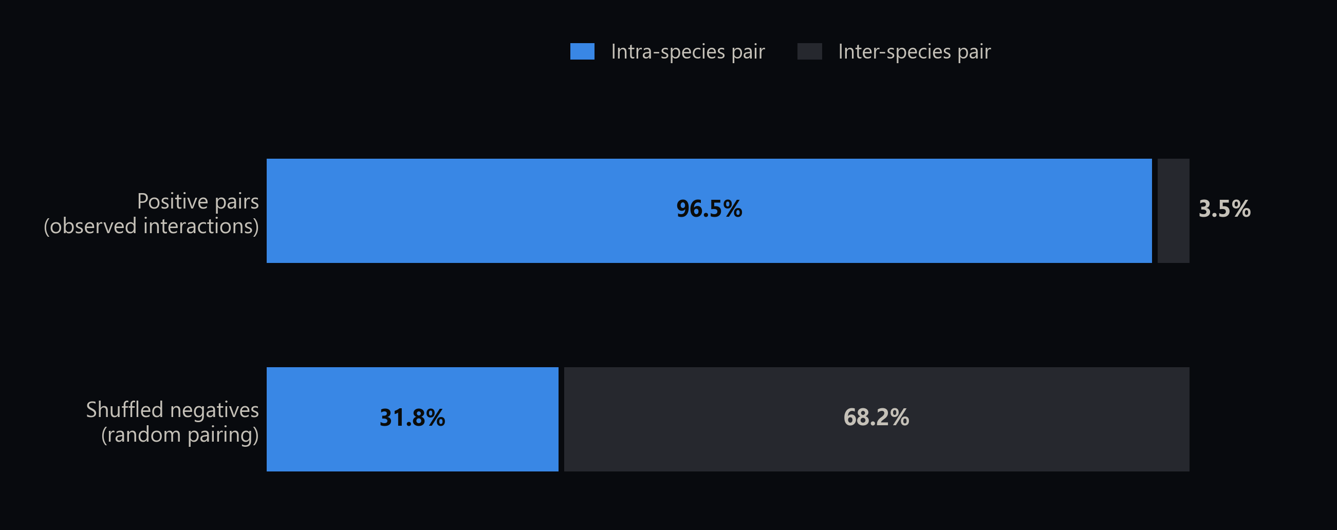
Interactions are studied within an organism. So positives inherit that structure: 96.5 percent of BioGRID positives are intra-species. Shuffling ignores the structure entirely and draws from the whole multi-species pool, which is 31.8 percent intra-species. The label and the taxonomy are now correlated, and the correlation is large.

How far the shortcut alone gets you

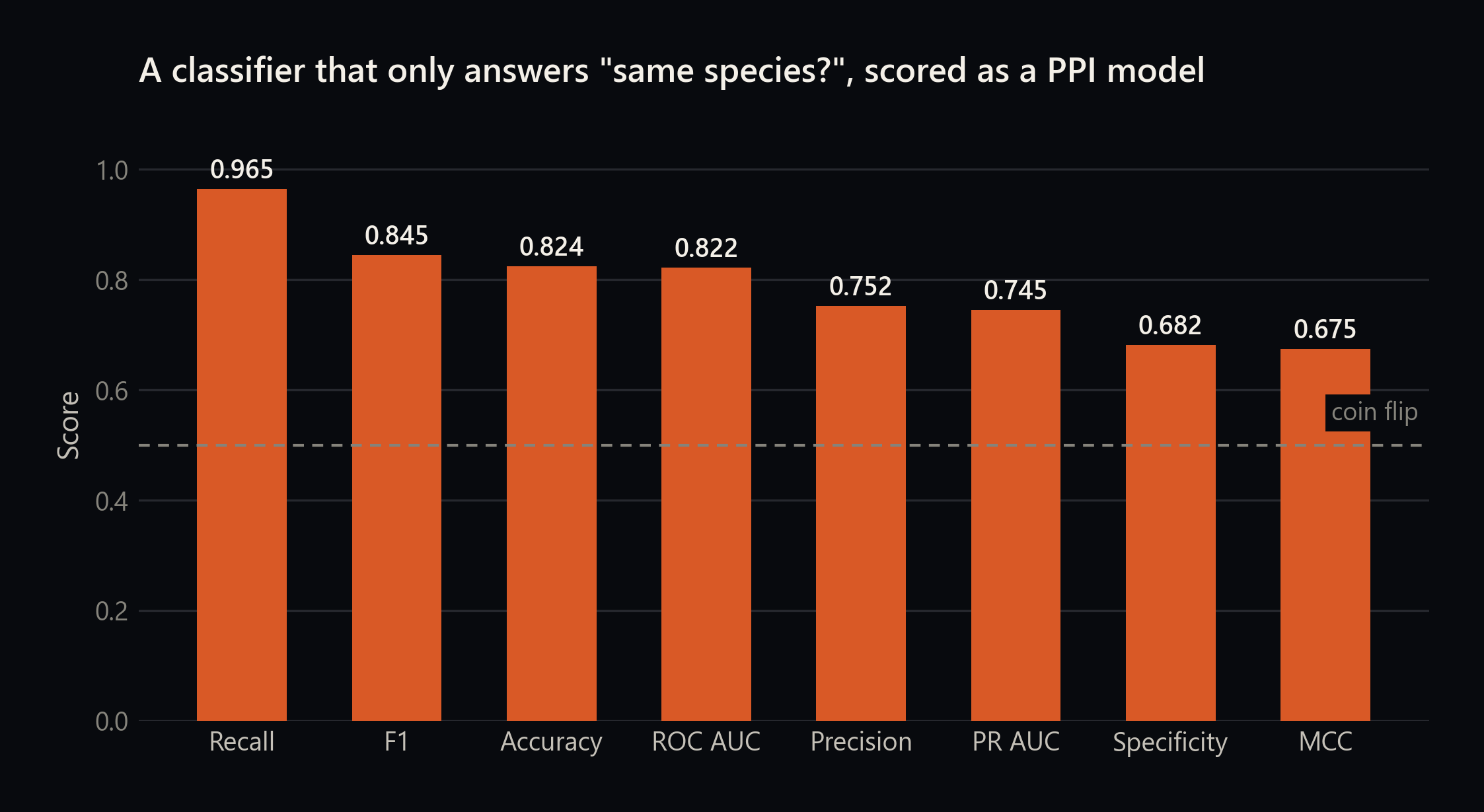
This is quantifiable without training anything. Simulate a classifier that has no idea what an interaction is and can only answer "same species?" Give it the BioGRID ratios, run it on a balanced set of 100,000 examples, and score it as if it were an interaction model.

Those are respectable-looking numbers. Any published result in that range on a shuffled-negative multi-species dataset is consistent with a model that has learned nothing about binding at all.

Can the model actually see taxonomy?

A shortcut only matters if the model can take it. So the second question is whether protein language model embeddings carry enough phylogenetic signal to support it.

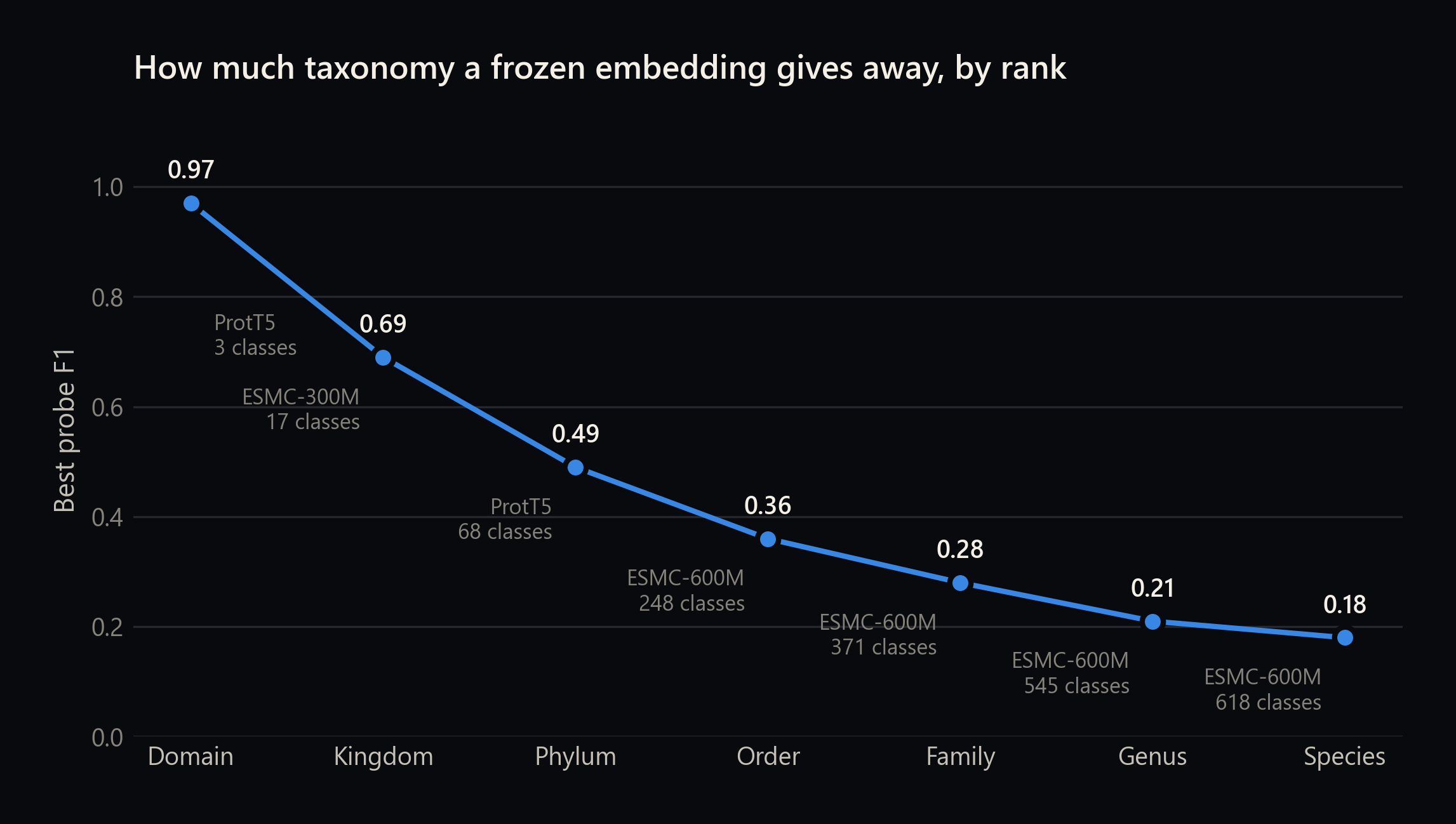
At the domain level this is nearly solved: 0.97 F1 across Archaea, Bacteria, and Eukarya. It degrades as the rank gets finer, down to 0.18 F1 across 618 species classes, which is far from reliable but far above the 0.00 a random baseline achieves.

Species-level classification is not the relevant test, though. Interaction models never see one protein; they see two. So the sharper probe is the paired binary question: given two sequences, are they from the same organism?

That is where the number gets uncomfortable. Most protein language models exceed 0.8 F1 on it, and ESMC-600M reaches 0.87. Even the homology controls exceed 0.7. The shortcut is not hypothetical. It is sitting in the embedding, ready to use.

Taking it away

The fix follows directly: when you build a negative, draw the two proteins from the same species as the positive pair. Same-species sampling makes the negatives taxonomically indistinguishable from the positives, so the shortcut carries no information.

Five models per strategy are trained on matched datasets. Same 4,523,432 training examples, same balanced label distribution, same 76,045 unique sequences, same frozen ESMC-600M encoder. They differ only in how negatives were drawn.

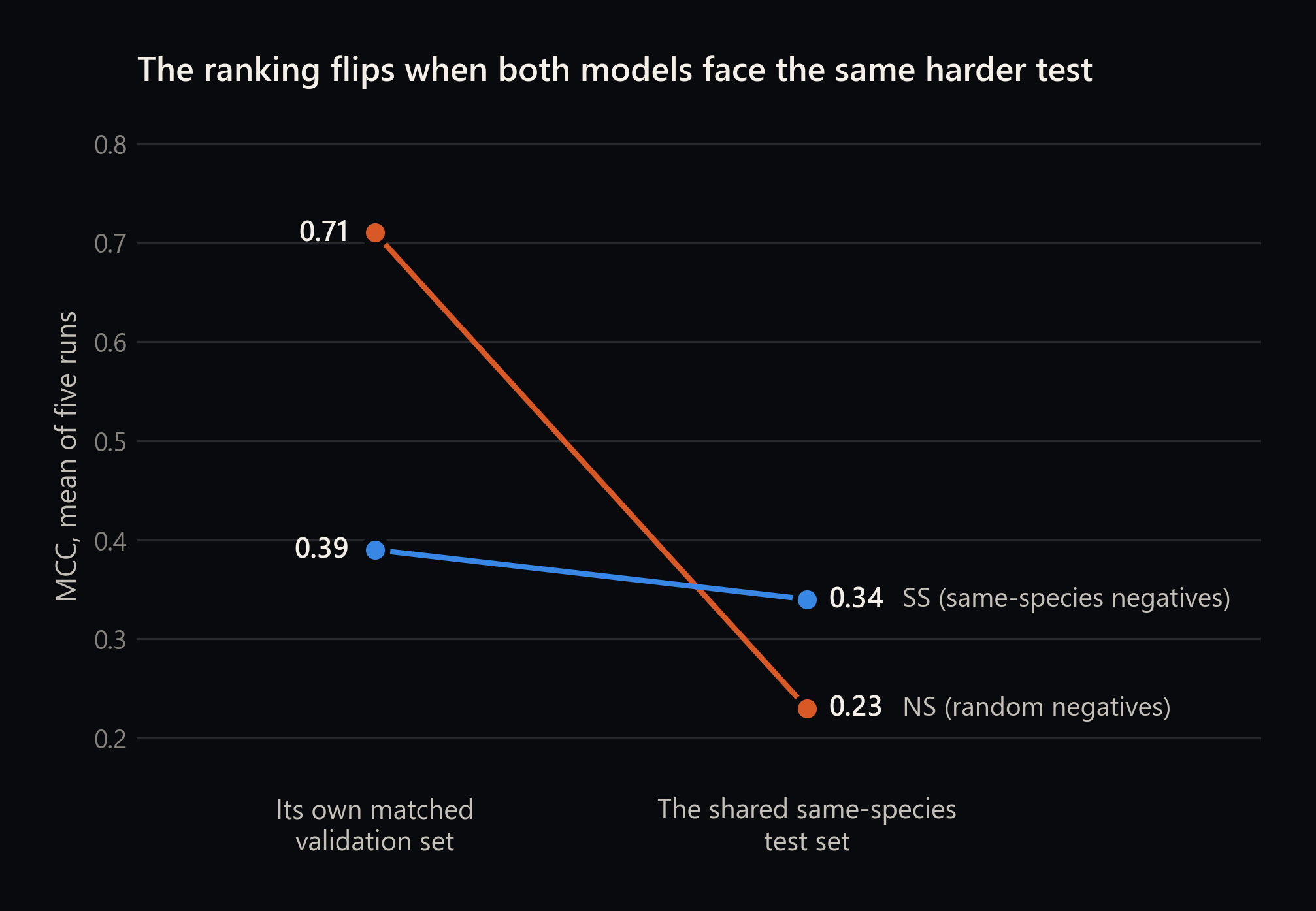
On its own validation set the random-negative model reports 0.71 MCC against the same-species model's 0.39, which would normally be read as a decisive win. On the shared same-species test set the ordering reverses: 0.23 against 0.34.

The training dynamics show the same thing from another angle. Random-negative models drive their average predicted probability on positives to 0.94, while same-species models plateau at 0.75. Both converge to roughly 0.5 on negatives. Confidently pushing positive logits up while remaining undecided on negatives is what reward hacking looks like when the reward has an exploitable seam in it.

The held-out check

One more evaluation, on a separate curated set with a taxonomy-aware split.

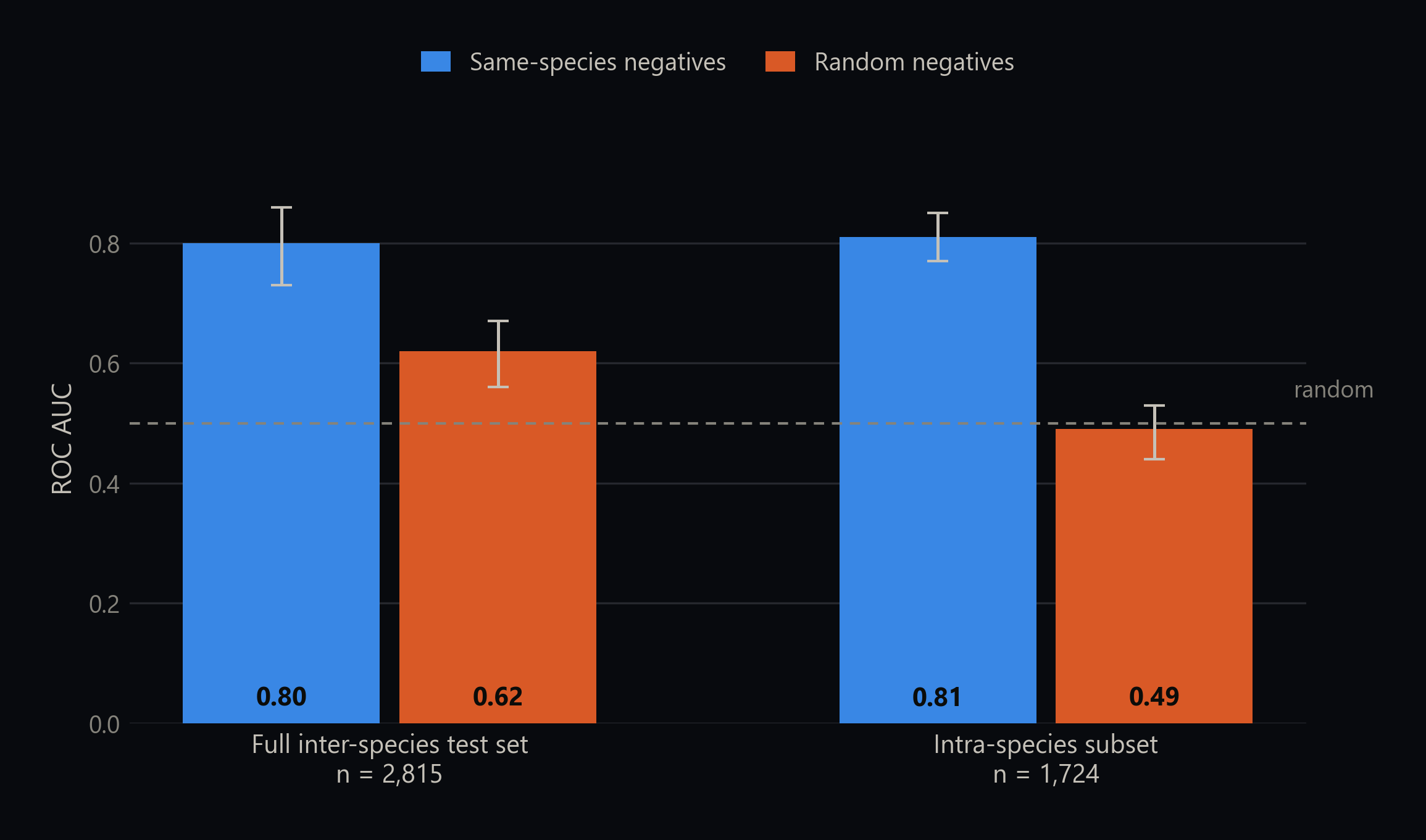
On the intra-species subset the same-species model reaches 0.81 ROC AUC and the random-negative model reaches 0.49, which is a coin flip (DeLong Z = 11.37, p below 10⁻¹⁵). Strip the taxonomy away and one model keeps working while the other stops entirely.

The result that cuts the other way

The obvious conclusion would be to stop using multi-species data. The opposite is true.

The best same-species multi-species model reaches 0.37 MCC, roughly 23 percent above the best reported result on the leakage-controlled single-species Bernett benchmark (0.30 MCC). So multi-species data does help, once the sampling is fixed. The problem was never the diversity. It was the seam that diversity opened up.

That comparison is suggestive rather than definitive. The two datasets draw from different sources (BioGRID against HIPPIE), roughly 45 percent of Bernett's positives overlap with BioGRID, and the multi-species set is substantially larger, so part of the gain could be scale rather than phylogenetic breadth. A size-matched control would separate the two.

Where both approaches fail

The most striking negative result is one neither strategy solves. On the held-out set, 1,091 positives were interspecies pairs, dominated by human-SARS-CoV-2 interactions. The same-species model called zero of them positive. The random-negative model called two. Both assigned them a mean probability near 0.46.

Host-pathogen interaction is among the most biomedically interesting corners of this field, and both models are simply blind to it. Same-species sampling fixes the confounder; it does not create competence on a task that was never in the training distribution. That gap is what Synteract-4's interspecies work goes after directly, and even there the result is clearing the random floor rather than solving the problem.

The general lesson

The pattern is clearest in interaction prediction because the negatives have to be manufactured. It is not confined there.

Any supervised protein dataset can carry hidden correlation between labels and taxonomy, organism of origin, assay source, curation practice, or sequence redundancy. Enzyme classification, localization, stability, and phenotype labels can all inherit unwanted structure when one taxonomic region dominates one label.

The practical rule is short: if taxonomy could explain the label, control for taxonomy. And treat implausibly strong results with suspicion. Above roughly 0.95 AUC or 0.8 MCC on a rigorously constructed interaction dataset, leakage or a confounder is the more likely explanation than a breakthrough.

This is also why a model description should not stop at the architecture. The data design is part of the model's behavior, and it is usually the part that decides what the model actually learned.